varexternalinstrument
varexternalinstrument.RmdBasic usage
The library is designed to work with the R vars package, though an interface is available to work with a generic set of reduced form residuals.
The package includes the replication data from Gertler Karadi (the original data can be found here).
The library integrates easily with the vars package. The following example illustrates how to replicate the main result from Gertler and Karadi (2015).
library(vars)
library(varexternalinstrument)

data(GKdata)

gkvar <- VAR(GKdata[, c("logip", "logcpi", "gs1", "ebp")], p = 12, type = "const")
shockcol <- externalinstrument(gkvar, GKdata$ff4_tc, "gs1")
shockcol
#>       logip      logcpi         gs1         ebp
#>  0.02886238 -0.03275585  0.19549144  0.11296773
The result, shockcol contains the instaneous response of each of the variables in the VAR to a shock to gs1 (in this case, the monetary policy indicator). This can then be used to create IRFs, etc.
Creating IRFs
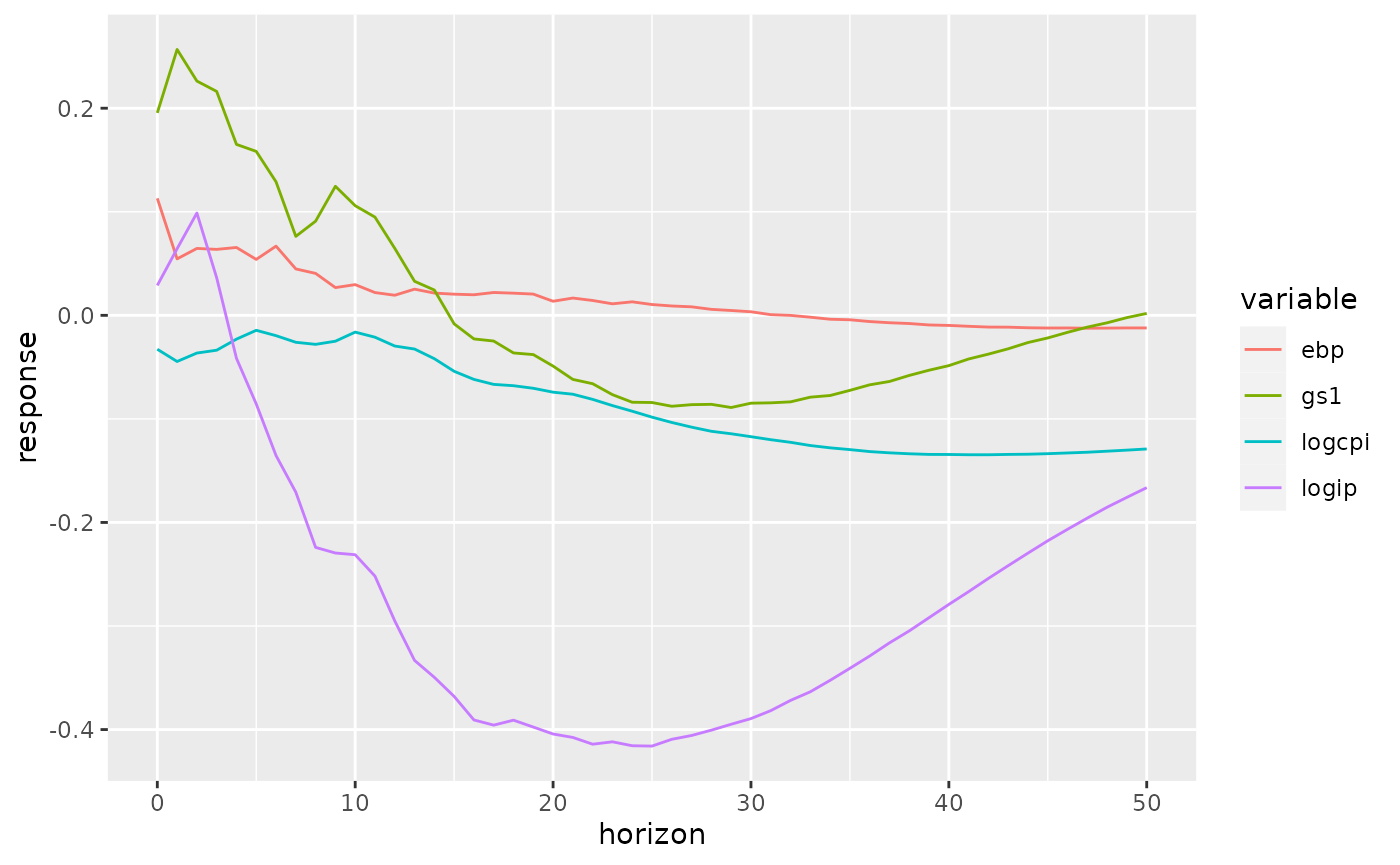
Here I use the Phi function from the vars package, which gives the moving average representation of an estimated var over a given finite horizon. I construct 20 period IRFs, mimicking figure 1 from Gertler & Karadi (2015).
library(tidyr)
library(dplyr)
library(ggplot2)
ma_representation <- Phi(gkvar, 50)
irfs <- apply(ma_representation, 3, function(x) x %*% shockcol)
irfs <- as.data.frame(t(irfs))
colnames(irfs) <- names(shockcol)
irfs <- mutate(irfs, horizon = 0:50)
irfs <- gather(irfs, key = variable, value = response, -horizon)
ggplot(irfs, aes(x = horizon, y = response, group = variable, color = variable)) + geom_line()